David Allen, London Natural History Society and GiGL Volunteer
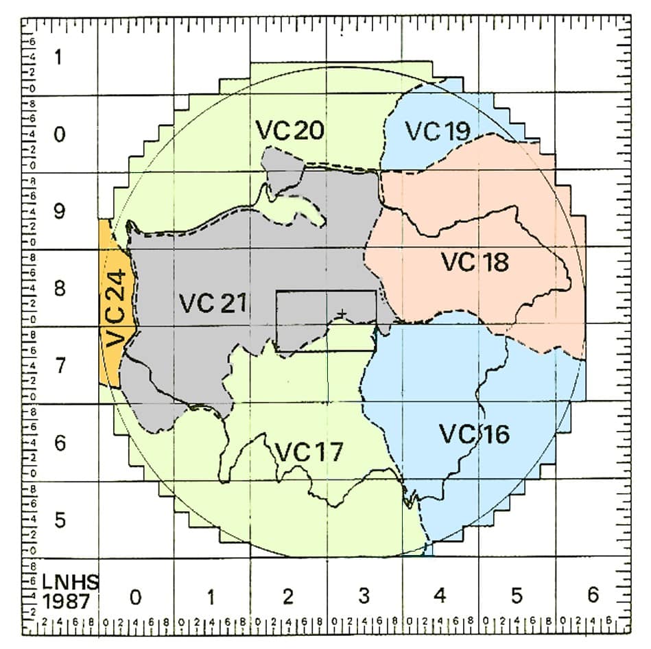
Map of Watsonian Vice-counties covering the LNHS recording area © LNHS 2019
Place has been an integral part of natural history observations from the very beginning. Authors have described the natural history of their parish, their town or their county often in great detail. But the systematic recording of place to give an account of distribution is much more recent. The idea of recording plants in Britain on a systematic basis by county goes back to the 1830s and was popularised by H. C. Watson in his Cybele Britannica of 1852; Watson established the idea of vice-counties for biological recording, dividing Britain into 112 more or less equal areas.
Much of this evolution of geographical recording boundaries can be well traced through the biological recording history of the London Natural History Society (LNHS).
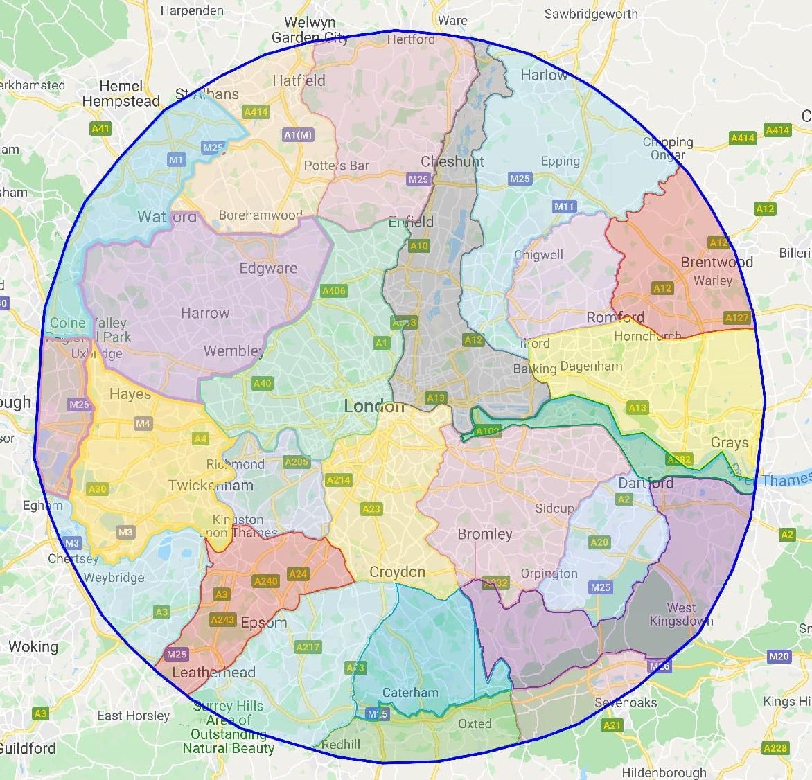
The twenty-four recording divisions within a 20-mile radius from St. Paul’s Cathedral © Google Maps 2019
The first defined recording area for LNHS was established in 1904, by the North London Natural History Society. Their area of operations was defined as being within a 20-mile radius from St. Paul’s Cathedral, north of the Thames, and was organised into twelve “Divisions”. On amalgamation with the City of London Entomological and Natural History Society in 1913 to form the London Natural History Society, the recording boundary was extended south of the river to complete the circle, with twelve matching southern divisions.
Thus the LNHS recording area included all of the City of London and the county of Middlesex, as well as parts of the administrative counties of Essex, Kent, Surrey, Buckinghamshire and Hertfordshire. The divisions were in essence habitat zones defined as far as possible by boundaries which could be walked. Additionally, there was a rectangular division for Inner London centred on Charing Cross.
LNHS bird records were first collected systematically in 1908 and plant records in 1917. With the establishment of recording divisions, the locations of these botanical and ornithological observations were allocated to a division, both on paper records and on herbarium sheets.
Hectads, tetrads and everything in-between
By the 1930s LNHS ornithologists had abandoned divisions in favour of vice-counties. The botanists carried on into the 1940s until vice-county recording for plants was introduced in 1942. In 1946 D. H. Kent began revising all the paper records and herbarium sheets and allocated each to a vice-county; vice-counties have been used to organise and present these records ever since. However, vice-counties are not the only recording boundaries adopted by biological recorders, as the years following the Second World War show an enormous acceleration in the application of mapping to natural history.
British National Grid
In 1946 the Ordnance Survey first printed the National Grid of 1km squares on Ordnance Survey maps. This was the culmination of a process begun in 1919 when the “British Grid System” was adopted on military maps. The grid could be used to specify points on a map economically, using a limited number of characters: a grid reference. This avoided the cumbersome notation of geographical coordinates and even more importantly, be used to define areas. A 1km square of the grid could be expressed using two letters and four digits (e.g. TQ1585); a 100m by 100m square using two letters and 6 digits (e.g. TQ156851).
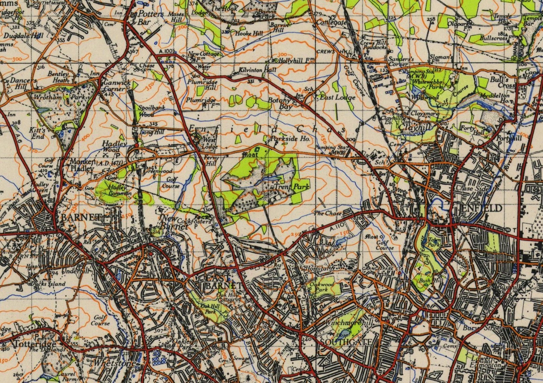
1km grid squares printed on OS One-inch England and Wales, New Popular Edition, 1945-47
© Reproduced with the permission of the National Library of Scotland
Hectads
In 1950 the Botanical Society of the British Isles (BSBI) published The Study of the Distribution of British Plants which laid the groundwork for the first atlas of the British flora; in this atlas, plant distribution was recorded by 10km grid squares – the hectad. Record collection began in 1954 and in 1962, the Atlas of the British Flora edited by Franklyn Perring and S. Max Walters was published. An interactive Atlas based on this data and more, can be found here.
This exemplified two post-war developments; the National Grid, and the use of 40 column-punched cards for recording. Observers wrote the details of the observation on the card, coders then punched holes in the cards to code species and location details. The cards could then be machine sorted and collated to give the distribution of species by 10km square. This is the first example of computer mapping published in Britain. The Atlas, and the punch cards used to record its data, are featured in an exhibition at the Computer History Museum in California, USA.
Tetrads
Problems of resolution, that is to say the scale at which observations were recorded, were next addressed in 1963, the year after the publication of the atlas. The discussion of local floras in the 1951 BSBI conference recommended the use of “tetrads” for local recording. A tetrad is a 2km by 2km set of grid squares, meaning there are 25 tetrads to a 10km square and there is a convention for defining each tetrad by letter within a 10km square. The first published use of tetrads was J. G. Dony’s Flora of Hertfordshire in 1967.
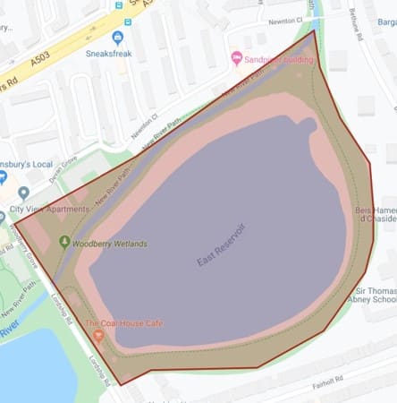
An example of a site polygon © Google maps 2019
Polygons
The “division” system originally used by the LNHS was an attempt to record observations by habitat type. Although grid recording is more precise, it is less hospitable to the “natural” classification of space.
However with the development of computing capacity, it becomes possible to define areas by a series of single locations defining a perimeter. This is the polygon. A nature reserve, for example, can be defined by its perimeter and enough computing power is available to recognise when any observational points fall within it, or indeed within any defined distance of it. This means an observation with a grid reference can be allocated to a known site.
What3words
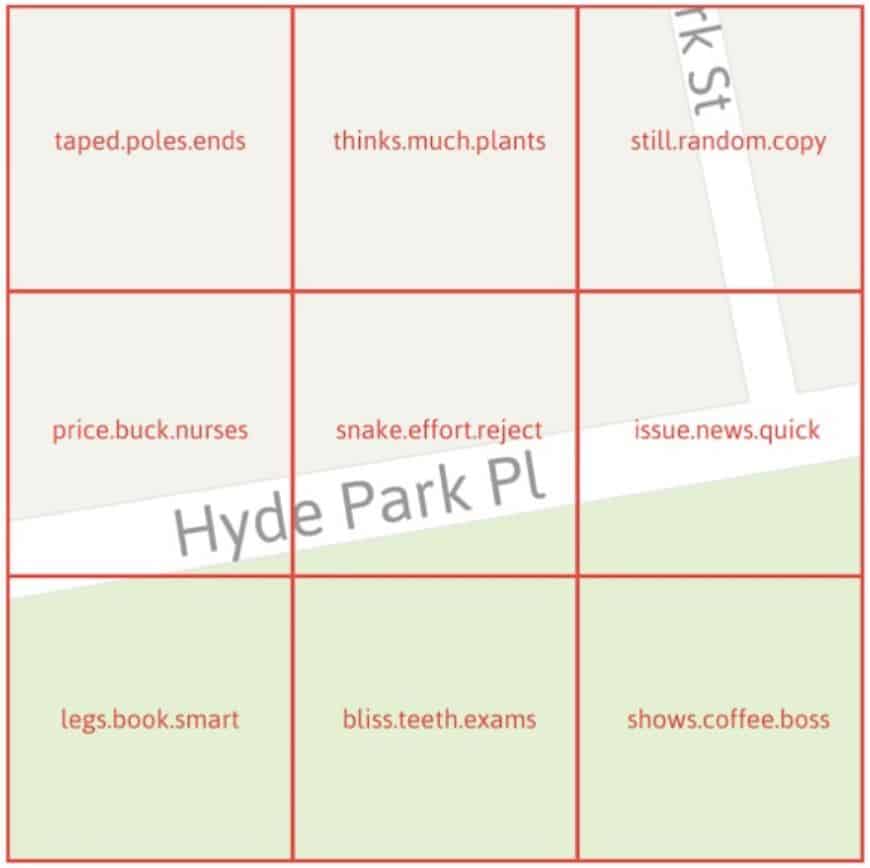
How what3words divide up areas © what3words.com
The latest geographical player to emerge is “what3words”. What3Words is “a geocode system for the communication of locations with a resolution of three metres…encod[ing] geographic coordinates into three dictionary words”. The system divides the globe into 17 trillion three metre squares, and each is given a name consisting of three dictionary words.
It is mindless, in that you cannot determine the relationship between any two locations on the basis of the code. However the code is much easier to record and to transmit without user error, and fuzzy logic comes into play when a code is searched for; something that would be impossible with numerical systems.
The system is still reliant on the accuracy of the satellite signal, but it is a useful way of pinpointing locations (invented by a roadie frustrated by drum kits always arriving at the wrong arena entrance). The entire system is designed to be used on a smartphone.
Resolving 17 trillion addresses into a meaningful coordinate is a relatively simple process with today’s computing power; grid reference or geographical coordinates. It remains to be seen how popular it becomes with the natural history community and who has the responsibility for resolving the locations.